Study Notes on Optimal Transport

最优运输问题

最优运输问题的目标就是以最小的成本将一个概率分布转换为另一个概率分布。即把概率分布 $\mathbf{c}$ 以最小的成本转换到概率分布 $\mathbf{r}$, 此时就要获得一个分配方案 $P \in \mathbb{R}^{n \times m}_{>0}$, 满足 $P \mathbf{1}_m = \mathbf{c}$ 和 $P^T \mathbf{1}_n = \mathbf{r}$。同时又要考虑运输成本：一个已知的成本矩阵$M$。于是最优传输问题可以表示为：

$$ \begin{gathered} d_M(\mathbf{r}, \mathbf{c}) = \min_{P \in U(\mathbf{r}, \mathbf{c})} \sum_{i,j} P_{i,j} M_{i,j}, \\ U(\mathbf{r}, \mathbf{c}) = \{ P \in \mathbb{R}^{n \times m}_{>0} | P \mathbf{1}_m = \mathbf{c}, P^T \mathbf{1}_n = \mathbf{r}\} \end{gathered} $$

此时 $d_M(\mathbf{r}, \mathbf{c})$ 被称为 Wasserstein metric 或者为 earth mover distance (EMD) 代价函数。

Sinkhorn 距离和 Sinkhorn 算法

Sinkhorn 距离是对前者 Wasserstein/EMD 距离的改进，引入了熵(Entropy)正则项：

$$ d^{\lambda}_M(\mathbf{r}, \mathbf{c}) = \min_{P \in U(\mathbf{r}, \mathbf{c})} \left( \sum_{i,j} P_{i,j} M_{i,j} - \frac{1}{\lambda} h(P) \right) $$

这里 $h(P) = -\sum_{i,j} P_{i,j} \log P_{i,j}$ 是P的信息熵，$\lambda$ 是正则项对应的超参。此时，求解这个优化问题：

$$ \begin{align*} & \mathcal{L} = \sum_{i,j} P_{i,j} M_{i,j} + \frac{1}{\lambda} \sum_{i,j} P_{i,j} \log P_{i,j} \\ \Rightarrow \quad & 0 = \frac{\partial \mathcal{L}}{\partial P_{i,j}} = M_{ij} + \frac{1}{\lambda} (P_{i,j} + 1) \\ \Rightarrow \quad & P_{i,j} = e^{-\lambda M_{ij} - 1} \end{align*} $$

这是在无约束条件下求得的 $P$ 的解，考虑约束条件的话，引入缩放因子 $\alpha_{i}$ 和 $\beta_{j}$ 用来让行和列满足约束：

$$ P_{i,j} = \alpha_{i} \beta_{j} e^{-\lambda M_{ij}} $$

最终的满足约束的 $P$ 的解可以通过下面这个伪代码和算法获得：

 1
 2
 3
 4
 5
 6
 7
 8
 9
10
11
12
13
14
15
16
17
18
19
20
21
22
23
24
25
26
27


def compute_optimal_transport(M, r, c, lam, epsilon=1e-8):
    """
    Computes the optimal transport matrix and Sinkhorn distance using 
    the Sinkhorn-Knopp algorithm
    Inputs:
        - M : cost matrix (n, m)
        - r : vector of marginals (n, )
        - c : vector of marginals (m, )
        - lam : strength of the entropic regularization
        - epsilon : convergence parameter
    Outputs:
        - P : optimal transport matrix (n, m)
        - dist : Sinkhorn distance
    """
    n, m = M.shape
    # initialize: P = e^{-\lambda * M} (P_{ij} = e^{-\lambda * M_{ij}})
    P = np.exp(- lam * M)
    P /= P.sum()
    u = np.zeros(n)
    # normalize this matrix
    while np.max(np.abs(u - P.sum(1))) > epsilon:
        # scale the rows such that the row sums match r
        u = P.sum(1)
        P *= (r / u).reshape((-1, 1)) 
        # scale the columns such that the column sums match c
        P *= (c / P.sum(0)).reshape((1, -1))
    return P, np.sum(P * M)

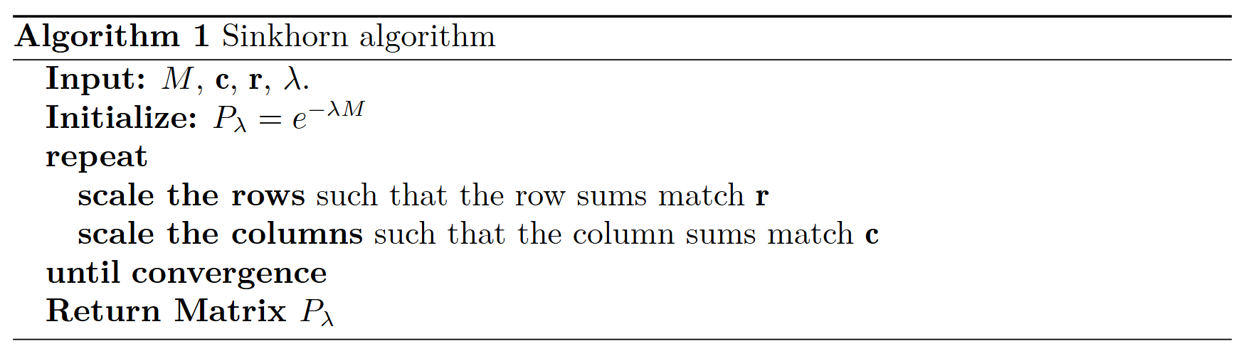
几何解释

最优传输问题，无论有没有熵正则化，都有一个漂亮的几何解释。

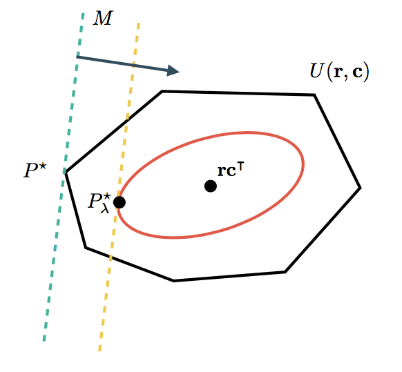
成本矩阵决定了分布的优劣方向。集合 $U(\mathbf{r}, \mathbf{c})$ 包含所有可行的分布。在未正则化的情况下，最优 $P^{\star}$ 通常在这样一个集合的某个角上。在添加熵正则因子时，我们将自己限制在熵最小的分布上，即位于平滑的红色曲线内。由于我们不必再处理 $U(\mathbf{r}, \mathbf{c})$ 的尖角，因此更容易找到最优值。特殊情况下，当 $\lambda \rightarrow \infty$ 时，$P_{\lambda}^{\star}$ 将变得越来越接近 $P^{\star}$（直到算法遇到数值困难）。另一方面，对于 $\lambda \rightarrow 0$ 的情况，只考虑熵项，$P_{\lambda}^{\star} = \mathbf{r} \mathbf{c}^T$（这是一种均匀分布，均匀分布信息熵最小）。

点击此处获取pdf版本。